Bayesian Function-on-Function Regression (FoFR)

2026-04-06

Introduction

This vignette provides a detailed guide to the fofr_bayes() function in the refundBayes package, which fits Bayesian Function-on-Function Regression (FoFR) models using Stan. FoFR extends both the scalar-on-function regression (SoFR) and function-on-scalar regression (FoSR) frameworks by modeling a functional response as a function of one or more functional predictors, along with optional scalar covariates.

In contrast to SoFR, where the outcome is scalar and the predictors are functional, and to FoSR, where the outcome is functional and the predictors are scalar, FoFR allows the effect of a functional predictor on a functional response to be captured through a bivariate coefficient function $\beta(s, t)$. The model is specified using the same mgcv-style syntax as the other regression functions in the refundBayes package.

The methodology extends the framework described in Jiang, Crainiceanu, and Cui (2025), Tutorial on Bayesian Functional Regression Using Stan, published in Statistics in Medicine.

Install the refundBayes Package

The refundBayes package can be installed from CRAN:

install.packages("refundBayes")

For the latest version of the refundBayes package, users can install from GitHub:

library(remotes)
remotes::install_github("https://github.com/ZirenJiang/refundBayes")

Statistical Model

The FoFR Model

Function-on-Function Regression (FoFR) models the relationship between a functional response and one or more functional predictors, optionally adjusted for scalar covariates. Both the response and the predictors are curves observed over (potentially different) continua.

For subject $i = 1, \ldots, n$, let $Y_i(t)$ be the functional response observed at time points $t = t_1, \ldots, t_M$ over a response domain $\mathcal{T}$, and let $\{W_i(s_l), s_l \in \mathcal{S}\}$ for $l = 1, \ldots, L$ be a functional predictor observed at $L$ points over a predictor domain $\mathcal{S}$. Let $\mathbf{X}_i = (X_{i1}, \ldots, X_{iP})^t$ be a $P \times 1$ vector of scalar predictors (the first covariate may be an intercept, $X_{i1} = 1$). The FoFR model assumes:

$$Y_i(t) = \sum_{p=1}^P X_{ip}\,\alpha_p(t) + \int_{\mathcal{S}} W_i(s)\,\beta(s, t)\,ds + e_i(t)$$

where:

• $\alpha_p(t)$ are functional coefficients for the scalar predictors, each describing how the $p$-th scalar predictor affects the response at each point $t \in \mathcal{T}$,
• $\beta(s, t)$ is the bivariate coefficient function that characterizes how the functional predictor at predictor-domain location $s$ affects the response at response-domain location $t$,
• $e_i(t)$ is the residual process, which is correlated across $t$.

The integral $\int_{\mathcal{S}} W_i(s)\,\beta(s, t)\,ds$ is approximated using a Riemann sum over the observed predictor-domain grid points. The domains $\mathcal{S}$ and $\mathcal{T}$ are not restricted to $[0,1]$; they are determined by the actual observation grids in the data.

When multiple functional predictors are present, the model extends naturally:

$$Y_i(t) = \sum_{p=1}^P X_{ip}\,\alpha_p(t) + \sum_{j=1}^J \int_{\mathcal{S}_j} W_{ij}(s)\,\beta_j(s, t)\,ds + e_i(t)$$

where $\beta_j(s, t)$ is the bivariate coefficient function for the $j$-th functional predictor.

Modeling the Residual Structure

To account for the within-subject correlation in the residuals, the model decomposes $e_i(t)$ using functional principal components, following the same approach as in FoSR (Goldsmith, Zipunnikov, and Schrack, 2015):

$$e_i(t) = \sum_{r=1}^R \xi_{ir}\,\phi_r(t) + \epsilon_i(t)$$

where $\phi_1(t), \ldots, \phi_R(t)$ are the eigenfunctions estimated via FPCA (using refund::fpca.face), $\xi_{ir}$ are the subject-specific FPCA scores with $\xi_{ir} \sim N(0, \lambda_r)$, and $\epsilon_i(t) \sim N(0, \sigma_\epsilon^2)$ is independent measurement error. The eigenvalues $\lambda_r$ and the error variance $\sigma_\epsilon^2$ are estimated from the data.

Scalar Predictor Coefficients via Penalized Splines

Each scalar predictor coefficient function $\alpha_p(t)$ is represented using $K$ spline basis functions $\psi_1(t), \ldots, \psi_K(t)$ in the response domain:

$$\alpha_p(t) = \sum_{k=1}^K a_{pk}\,\psi_k(t)$$

Smoothness is induced through a quadratic penalty:

$$p(\mathbf{a}_p) \propto \exp\left(-\frac{\mathbf{a}_p^t \mathbf{S} \mathbf{a}_p}{2\sigma_p^2}\right)$$

where $\mathbf{S}$ is the penalty matrix derived from the spline basis and $\sigma_p^2$ is the smoothing parameter for the $p$-th scalar predictor, estimated from the data.

Bivariate Coefficient via Tensor Product Basis

The key feature of FoFR is the bivariate coefficient function $\beta(s, t)$, which lives on the product domain $\mathcal{S} \times \mathcal{T}$. This function is represented using a tensor product of two sets of basis functions:

• Predictor-domain basis: $B_1(s), \ldots, B_Q(s)$, constructed from the s() term in the formula using the mgcv spline basis (e.g., cubic regression splines). These are further decomposed into random and fixed effect components via the spectral reparametrisation of mgcv::smooth2random(), yielding $\tilde{B}_1^r(s), \ldots, \tilde{B}_{Q_r}^r(s)$ (random effects) and $\tilde{B}_1^f(s), \ldots, \tilde{B}_{Q_f}^f(s)$ (fixed effects).

• Response-domain basis: $\psi_1(t), \ldots, \psi_K(t)$, the same spline basis used for the scalar predictor coefficients.

The bivariate coefficient is then:

$$\beta(s, t) = \sum_{k=1}^K \left[\sum_{q=1}^{Q_r} \theta_{qk}^r\,\tilde{B}_q^r(s) + \sum_{q=1}^{Q_f} \theta_{qk}^f\,\tilde{B}_q^f(s)\right] \psi_k(t)$$

where $\boldsymbol{\Theta}^r$ is the $Q_r \times K$ matrix of random effect coefficients and $\boldsymbol{\Theta}^f$ is the $Q_f \times K$ matrix of fixed effect coefficients.

With this representation, the integral contribution of the functional predictor becomes:

$$\int_{\mathcal{S}} W_i(s)\,\beta(s, t)\,ds \approx \left[\tilde{\mathbf{X}}_{i}^r \boldsymbol{\Theta}^r + \tilde{\mathbf{X}}_{i}^f \boldsymbol{\Theta}^f\right] \boldsymbol{\psi}(t)$$

where $\tilde{\mathbf{X}}_{i}^r$ and $\tilde{\mathbf{X}}_{i}^f$ are the $1 \times Q_r$ and $1 \times Q_f$ row vectors of the transformed predictor-domain design matrices for subject $i$ (the same matrices used in SoFR).

In matrix notation for all subjects, the functional predictor contribution to the mean is:

$$\left(\tilde{\mathbf{X}}^r \boldsymbol{\Theta}^r + \tilde{\mathbf{X}}^f \boldsymbol{\Theta}^f\right) \boldsymbol{\Psi}$$

which is an $n \times M$ matrix, where $\boldsymbol{\Psi}$ is the $K \times M$ matrix of response-domain spline basis evaluations.

Dual-Direction Smoothness Penalties

Because the bivariate coefficient $\beta(s, t)$ lives on a two-dimensional domain, smoothness must be enforced in both directions:

Predictor-domain smoothness ($s$-direction)

Following the same approach as in SoFR, the random effect coefficients use a variance-component reparametrisation:

$$\boldsymbol{\Theta}^r = \sigma_s \cdot \mathbf{Z}^r, \quad \text{vec}(\mathbf{Z}^r) \sim N(\mathbf{0}, \mathbf{I})$$

where $\sigma_s^2$ is the predictor-domain smoothing parameter. This is the standard non-centered parameterisation that separates the scale ($\sigma_s$) from the direction ($\mathbf{Z}^r$), improving sampling efficiency in Stan.

Response-domain smoothness ($t$-direction)

The response-domain penalty matrix $\mathbf{S}$ is applied row-wise to the coefficient matrices. For each row $q$ of $\boldsymbol{\Theta}^r$ and $\boldsymbol{\Theta}^f$:

$$p(\boldsymbol{\Theta}_q^r) \propto \exp\left(-\frac{\boldsymbol{\Theta}_q^r \mathbf{S}\,(\boldsymbol{\Theta}_q^r)^t}{2\sigma_t^2}\right), \qquad p(\boldsymbol{\Theta}_q^f) \propto \exp\left(-\frac{\boldsymbol{\Theta}_q^f \mathbf{S}\,(\boldsymbol{\Theta}_q^f)^t}{2\sigma_t^2}\right)$$

where $\sigma_t^2$ is the response-domain smoothing parameter. This ensures that $\beta(s, t)$ is smooth in the $t$-direction for every fixed $s$.

The two smoothing parameters $\sigma_s^2$ and $\sigma_t^2$ are estimated from the data with weakly informative inverse-Gamma priors.

Full Bayesian Model

The complete Bayesian FoFR model combines the mean structure, residual FPCA decomposition, and all priors:

$$\begin{cases} Y_i(t) = \boldsymbol{\mu}_i(t) + e_i(t), \quad i = 1, \ldots, n \\[6pt] \boldsymbol{\mu}_i(t) = \displaystyle\sum_{p=1}^P X_{ip}\,\alpha_p(t) + \int_{\mathcal{S}} W_i(s)\,\beta(s,t)\,ds \\[6pt] e_i(t) = \displaystyle\sum_{r=1}^R \xi_{ir}\,\phi_r(t) + \epsilon_i(t) \end{cases}$$

In matrix form for all subjects:

$$\mathbf{Y} = \mathbf{X}\,\mathbf{A}^t \boldsymbol{\Psi} + \left(\tilde{\mathbf{X}}^r \boldsymbol{\Theta}^r + \tilde{\mathbf{X}}^f \boldsymbol{\Theta}^f\right) \boldsymbol{\Psi} + \boldsymbol{\Xi}\,\boldsymbol{\Phi} + \boldsymbol{E}$$

where $\mathbf{Y}$ is the $n \times M$ matrix of functional responses, $\mathbf{X}$ is the $n \times P$ scalar design matrix, $\mathbf{A}$ is the $K \times P$ matrix of scalar predictor spline coefficients, $\boldsymbol{\Xi}$ is the $n \times R$ matrix of FPCA scores, and $\boldsymbol{\Phi}$ is the $R \times M$ matrix of eigenfunctions.

Prior Specification

The full prior specification is:

Parameter	Prior	Description
$\mathbf{a}_p$ (scalar predictor spline coefs)	$p(\mathbf{a}_p) \propto \exp\left(-\frac{\mathbf{a}_p^t \mathbf{S}\,\mathbf{a}_p}{2\sigma_p^2}\right)$	Penalized spline prior for smoothness of $\alpha_p(t)$
$\sigma_p^2$ (scalar smoothing parameter)	$\sigma_p^2 \sim \text{Inv-Gamma}(0.001, 0.001)$	Weakly informative prior on smoothing
$\text{vec}(\mathbf{Z}^r)$ (standardized random effects)	$\text{vec}(\mathbf{Z}^r) \sim N(\mathbf{0}, \mathbf{I})$	Non-centered parameterisation for $s$-direction
$\sigma_s^2$ (predictor-domain smoothing)	$\sigma_s^2 \sim \text{Inv-Gamma}(0.0005, 0.0005)$	Prior on predictor-domain smoothing
$\boldsymbol{\Theta}_q^r, \boldsymbol{\Theta}_q^f$ (row-wise)	$p(\boldsymbol{\Theta}_q) \propto \exp\left(-\frac{\boldsymbol{\Theta}_q \mathbf{S}\,\boldsymbol{\Theta}_q^t}{2\sigma_t^2}\right)$	Penalized spline prior for response-domain smoothness
$\sigma_t^2$ (response-domain smoothing)	$\sigma_t^2 \sim \text{Inv-Gamma}(0.001, 0.001)$	Prior on response-domain smoothing
$\xi_{ir}$ (FPCA scores)	$\xi_{ir} \sim N(0, \lambda_r)$	FPCA score distribution
$\lambda_r$ (FPCA eigenvalues)	$\lambda_r^2 \sim \text{Inv-Gamma}(0.001, 0.001)$	Weakly informative prior on eigenvalues
$\sigma_\epsilon^2$ (residual variance)	$\sigma_\epsilon^2 \sim \text{Inv-Gamma}(0.001, 0.001)$	Weakly informative prior on noise variance

Likelihood

The likelihood for the functional response is Gaussian:

$$\log p(\mathbf{Y} \mid \boldsymbol{\mu}, \sigma_\epsilon^2) = -\frac{nM}{2}\log\sigma_\epsilon - \frac{1}{2\sigma_\epsilon^2}\sum_{i=1}^n \sum_{m=1}^M \{Y_i(t_m) - \mu_i(t_m)\}^2$$

where the mean function $\mu_i(t_m)$ includes contributions from scalar predictors, functional predictors, and FPCA scores.

Optional: Joint FPCA Modeling

The default fofr_bayes() model treats the observed functional predictor $W_i(s)$ as if it were observed without error. When the predictor curves are noisy, this attenuates the bivariate coefficient $\beta(s,t)$ toward zero (errors-in-variables bias) and shrinks the credible-band width. The joint_FPCA argument activates an alternative model in which $W_i(s)$ is replaced by an FPCA representation and the subject-specific FPC scores are sampled jointly with the bivariate coefficient, propagating the FPCA uncertainty into the posterior of $\beta(s,t)$.

The same joint_FPCA argument is available in sofr_bayes() and fcox_bayes(). The full model specification (FPCA likelihood for the predictor, FPC-score prior centered on the initial refund::fpca.sc() scores, the resulting Stan program with bivariate coefficients in the FPC basis, and a worked FoFR example) is presented in the dedicated Joint FPCA vignette.

Relationship to SoFR and FoSR

The FoFR model nests both the SoFR and FoSR models as special cases:

Model	Response	Predictors	Coefficient	Implemented in
SoFR	Scalar $Y_i$	Functional $W_i(s)$	Univariate $\beta(s)$	sofr_bayes()
FoSR	Functional $Y_i(t)$	Scalar $X_{ip}$	Univariate $\alpha_p(t)$	fosr_bayes()
FoFR	Functional $Y_i(t)$	Functional $W_i(s)$ + Scalar $X_{ip}$	Bivariate $\beta(s,t)$ + Univariate $\alpha_p(t)$	fofr_bayes()

The fofr_bayes() function inherits:

• From FoSR: the response-domain spline basis $\boldsymbol{\Psi}$, the FPCA residual structure, and the scalar predictor handling.
• From SoFR: the predictor-domain spectral reparametrisation (random/fixed effect decomposition via mgcv::smooth2random()), the basis extraction, and the functional coefficient reconstruction.

The fofr_bayes() Function

Usage

fofr_bayes(
  formula,
  data,
  joint_FPCA = NULL,
  runStan = TRUE,
  niter = 3000,
  nwarmup = 1000,
  nchain = 3,
  ncores = 1,
  spline_type = "bs",
  spline_df = 10
)

Arguments

Argument	Description
formula	Functional regression formula, using the same syntax as mgcv::gam. The left-hand side is the functional response (an $n \times M$ matrix in data). The right-hand side includes scalar predictors as standard terms and functional predictors via s(..., by = ...) terms. At least one functional predictor must be present; otherwise use fosr_bayes().
data	A data frame containing all variables used in the model. The functional response and functional predictor should be stored as $n \times M$ and $n \times L$ matrices, respectively.
joint_FPCA	A logical (TRUE/FALSE) vector of the same length as the number of functional predictors, indicating whether to jointly model FPCA for each functional predictor. When TRUE, the observed functional predictor is replaced by an FPCA representation and its FPC scores are sampled jointly with the bivariate coefficient (errors-in-variables-aware fit). See the Joint FPCA vignette for the model specification and a worked FoFR example. Default is NULL, which sets all entries to FALSE (no joint FPCA).
runStan	Logical. Whether to run the Stan program. If FALSE, the function only generates the Stan code and data without sampling. This is useful for inspecting or modifying the generated Stan code. Default is TRUE.
niter	Total number of Bayesian posterior sampling iterations (including warmup). Default is 3000.
nwarmup	Number of warmup (burn-in) iterations. These samples are discarded and not used for inference. Default is 1000.
nchain	Number of Markov chains for posterior sampling. Multiple chains help assess convergence. Default is 3.
ncores	Number of CPU cores to use when executing the chains in parallel. Default is 1.
spline_type	Type of spline basis used for the response-domain component. Default is "bs" (B-splines). Other types supported by mgcv may also be used.
spline_df	Number of degrees of freedom (basis functions) for the response-domain spline basis. Default is 10.

Return Value

The function returns a list of class "refundBayes" containing the following elements:

Element	Description
stanfit	The Stan fit object (class stanfit). Can be used for convergence diagnostics, traceplots, and additional summaries via the rstan package.
spline_basis	Basis functions used to reconstruct the functional coefficients from the posterior samples.
stancode	A character string containing the generated Stan model code.
standata	A list containing the data passed to the Stan model.
scalar_func_coef	A 3-d array ($Q \times P \times M$) of posterior samples for scalar predictor coefficient functions $\alpha_p(t)$, where $Q$ is the number of posterior samples, $P$ is the number of scalar predictors, and $M$ is the number of response-domain time points. NULL if no scalar predictors.
bivar_func_coef	A list of 3-d arrays. Each element corresponds to one functional predictor and is an array of dimension $Q \times L \times M$, representing posterior samples of the bivariate coefficient function $\beta(s, t)$ evaluated on the predictor-domain grid ($L$ points) and response-domain grid ($M$ points).
func_coef	Same as scalar_func_coef; included for compatibility with the plot.refundBayes() method.
family	The model family: "fofr".

Formula Syntax

The formula combines the FoSR syntax (functional response on the left-hand side) with the SoFR syntax (functional predictors via s() terms on the right-hand side):

Y_mat ~ X1 + X2 + s(sindex, by = X_func, bs = "cr", k = 10)

where:

• Y_mat: the name of the functional response variable in data. This should be an $n \times M$ matrix, where each row contains the functional observations for one subject across $M$ response-domain time points.
• X1, X2: scalar predictor(s), included using standard formula syntax.
• s(sindex, by = X_func, bs = "cr", k = 10): the functional predictor term:
  • sindex: an $n \times L$ matrix of predictor-domain grid points. Each row contains the same $L$ observation points (replicated across subjects).
  • X_func: an $n \times L$ matrix of functional predictor values. The $i$-th row contains the $L$ observed values for subject $i$.
  • bs: the type of spline basis for the predictor domain (e.g., "cr" for cubic regression splines).
  • k: the number of basis functions in the predictor domain.

The response-domain spline basis is controlled separately via the spline_type and spline_df arguments to fofr_bayes(). This design separates the two basis specifications: the predictor-domain basis is specified in the formula (as in SoFR), while the response-domain basis is specified via function arguments (as in FoSR).

Multiple functional predictors can be included by adding additional s() terms.

Example: Bayesian FoFR with Simulated Data

We demonstrate the fofr_bayes() function using a simulation study with a known bivariate coefficient function $\beta(s, t)$ and a scalar predictor coefficient function $\alpha(t)$.

Simulate Data

library(refundBayes)

set.seed(42)

# --- Dimensions ---
n  <- 200   # number of subjects
L  <- 30    # number of predictor-domain grid points
M  <- 30    # number of response-domain grid points

sindex <- seq(0, 1, length.out = L)   # predictor domain grid
tindex <- seq(0, 1, length.out = M)   # response domain grid

# --- Functional predictor X(s): smooth random curves ---
X_func <- matrix(0, nrow = n, ncol = L)
for (i in 1:n) {
  X_func[i, ] <- rnorm(1) * sin(2 * pi * sindex) +
                 rnorm(1) * cos(2 * pi * sindex) +
                 rnorm(1) * sin(4 * pi * sindex) +
                 rnorm(1, sd = 0.3)
}

# --- Scalar predictor ---
age <- rnorm(n)

# --- True coefficient functions ---
# Bivariate coefficient: beta(s, t) = sin(2*pi*s) * cos(2*pi*t)
beta_true <- outer(sin(2 * pi * sindex), cos(2 * pi * tindex))

# Scalar coefficient function: alpha(t) = 0.5 * sin(pi*t)
alpha_true <- 0.5 * sin(pi * tindex)

# --- Generate functional response ---
# Y_i(t) = age_i * alpha(t) + integral X_i(s) beta(s,t) ds + epsilon_i(t)
signal_scalar <- outer(age, alpha_true)                    # n x M
signal_func   <- (X_func %*% beta_true) / L               # n x M  (Riemann sum)
epsilon        <- matrix(rnorm(n * M, sd = 0.3), nrow = n) # n x M

Y_mat <- signal_scalar + signal_func + epsilon

# --- Organize data ---
dat <- data.frame(age = age)
dat$Y_mat  <- Y_mat
dat$X_func <- X_func
dat$sindex <- matrix(rep(sindex, n), nrow = n, byrow = TRUE)

The simulated dataset dat contains:

• Y_mat: an $n \times M$ matrix of functional response values,
• age: a scalar predictor,
• X_func: an $n \times L$ matrix of functional predictor values (smooth random curves),
• sindex: an $n \times L$ matrix of predictor-domain grid points (identical rows).

The true data-generating model is: $$Y_i(t) = \text{age}_i \cdot 0.5\sin(\pi t) + \frac{1}{L}\sum_{l=1}^L X_i(s_l)\,\sin(2\pi s_l)\cos(2\pi t) + \epsilon_i(t), \quad \epsilon_i(t) \sim N(0, 0.3^2)$$

Fit the Bayesian FoFR Model

fit_fofr <- fofr_bayes(
  formula     = Y_mat ~ age + s(sindex, by = X_func, bs = "cr", k = 10),
  data        = dat,
  spline_type = "bs",
  spline_df   = 10,
  niter       = 2000,
  nwarmup     = 1000,
  nchain      = 3,
  ncores      = 3
)

In this call:

• The formula specifies the functional response Y_mat (an $n \times M$ matrix) with one scalar predictor age and one functional predictor X_func.
• The predictor-domain spline basis uses cubic regression splines (bs = "cr") with k = 10 basis functions.
• The response-domain spline basis uses B-splines (spline_type = "bs") with spline_df = 10 degrees of freedom.
• The eigenfunctions for the residual structure are estimated automatically via FPCA using refund::fpca.face.
• The sampler runs 3 chains in parallel, each with 2000 total iterations (1000 warmup + 1000 posterior samples).

A Note on Computation

FoFR models are the most computationally demanding among the models in refundBayes because the Stan program estimates bivariate coefficient matrices (with $Q_r \times K + Q_f \times K$ parameters per functional predictor) in addition to the scalar predictor coefficients and FPCA scores. For exploratory analyses, consider using fewer basis functions (e.g., k = 5, spline_df = 5) and a single chain. For final inference, use the full setup with multiple chains and convergence diagnostics.

Visualisation

Bivariate Coefficient $\hat{\beta}(s, t)$

The estimated bivariate coefficient $\hat{\beta}(s,t)$ is stored as a 3-d array in bivar_func_coef. The posterior mean surface and comparison with the truth can be visualised using heatmaps:

# Posterior mean of the bivariate coefficient
beta_est  <- apply(fit_fofr$bivar_func_coef[[1]], c(2, 3), mean)

# Pointwise 95% credible interval bounds
beta_lower <- apply(fit_fofr$bivar_func_coef[[1]], c(2, 3),
                    function(x) quantile(x, 0.025))
beta_upper <- apply(fit_fofr$bivar_func_coef[[1]], c(2, 3),
                    function(x) quantile(x, 0.975))

# Side-by-side heatmaps: true vs estimated vs difference
par(mfrow = c(1, 3), mar = c(4, 4, 2, 1))
image(sindex, tindex, beta_true,
      xlab = "s (predictor domain)", ylab = "t (response domain)",
      main = expression("True " * beta(s, t)),
      col = hcl.colors(64, "Blue-Red 3"))
image(sindex, tindex, beta_est,
      xlab = "s (predictor domain)", ylab = "t (response domain)",
      main = expression("Estimated " * hat(beta)(s, t)),
      col = hcl.colors(64, "Blue-Red 3"))
image(sindex, tindex, beta_est - beta_true,
      xlab = "s (predictor domain)", ylab = "t (response domain)",
      main = "Difference (Est - True)",
      col = hcl.colors(64, "Blue-Red 3"))

For richer 3-d surface visualisations, use fields::image.plot() or plotly::plot_ly() with type "surface".

Scalar Coefficient Function $\hat{\alpha}(t)$

The estimated scalar predictor coefficient function can be plotted with pointwise credible intervals:

alpha_est   <- apply(fit_fofr$scalar_func_coef[, 1, ], 2, mean)
alpha_lower <- apply(fit_fofr$scalar_func_coef[, 1, ], 2,
                     function(x) quantile(x, 0.025))
alpha_upper <- apply(fit_fofr$scalar_func_coef[, 1, ], 2,
                     function(x) quantile(x, 0.975))

par(mfrow = c(1, 1))
plot(tindex, alpha_true, type = "l", lwd = 2, col = "black",
     ylim = range(c(alpha_lower, alpha_upper)),
     xlab = "t (response domain)", ylab = expression(alpha(t)),
     main = "Scalar coefficient function: age")
lines(tindex, alpha_est, col = "blue", lwd = 2)
polygon(c(tindex, rev(tindex)),
        c(alpha_lower, rev(alpha_upper)),
        col = rgb(0, 0, 1, 0.2), border = NA)
legend("topright",
       legend = c("Truth", "Posterior mean", "95% CI"),
       col = c("black", "blue", rgb(0, 0, 1, 0.2)),
       lwd = c(2, 2, 10), bty = "n")

Slices of the Bivariate Coefficient

To examine $\beta(s, t)$ at fixed values of $s$ or $t$, extract slices from the posterior:

# Fix s at the midpoint of the predictor domain and plot beta(s_mid, t)
s_mid_idx <- which.min(abs(sindex - 0.5))

beta_slice_est   <- apply(fit_fofr$bivar_func_coef[[1]][, s_mid_idx, ], 2, mean)
beta_slice_lower <- apply(fit_fofr$bivar_func_coef[[1]][, s_mid_idx, ], 2,
                          function(x) quantile(x, 0.025))
beta_slice_upper <- apply(fit_fofr$bivar_func_coef[[1]][, s_mid_idx, ], 2,
                          function(x) quantile(x, 0.975))
beta_slice_true  <- beta_true[s_mid_idx, ]

plot(tindex, beta_slice_true, type = "l", lwd = 2, col = "black",
     ylim = range(c(beta_slice_lower, beta_slice_upper)),
     xlab = "t (response domain)",
     ylab = expression(beta(s[mid], t)),
     main = paste0("Slice at s = ", round(sindex[s_mid_idx], 2)))
lines(tindex, beta_slice_est, col = "red", lwd = 2)
polygon(c(tindex, rev(tindex)),
        c(beta_slice_lower, rev(beta_slice_upper)),
        col = rgb(1, 0, 0, 0.2), border = NA)
legend("topright",
       legend = c("Truth", "Posterior mean", "95% CI"),
       col = c("black", "red", rgb(1, 0, 0, 0.2)),
       lwd = c(2, 2, 10), bty = "n")

Numerical Summary

# RMSE of the bivariate coefficient surface
cat("RMSE of beta(s,t):", sqrt(mean((beta_est - beta_true)^2)), "\n")

# RMSE of the scalar coefficient function
cat("RMSE of alpha(t): ", sqrt(mean((alpha_est - alpha_true)^2)), "\n")

Inspecting the Generated Stan Code

Setting runStan = FALSE allows you to inspect or modify the Stan code before running the model:

# Generate Stan code without running the sampler
fofr_code <- fofr_bayes(
  formula     = Y_mat ~ age + s(sindex, by = X_func, bs = "cr", k = 10),
  data        = dat,
  spline_type = "bs",
  spline_df   = 10,
  runStan     = FALSE
)

# Print the generated Stan code
cat(fofr_code$stancode)

The generated Stan code includes all five standard blocks (data, transformed data, parameters, transformed parameters, model). The parameters block declares matrix-valued parameters for the bivariate coefficients, and the model block includes both $s$-direction and $t$-direction smoothness priors.

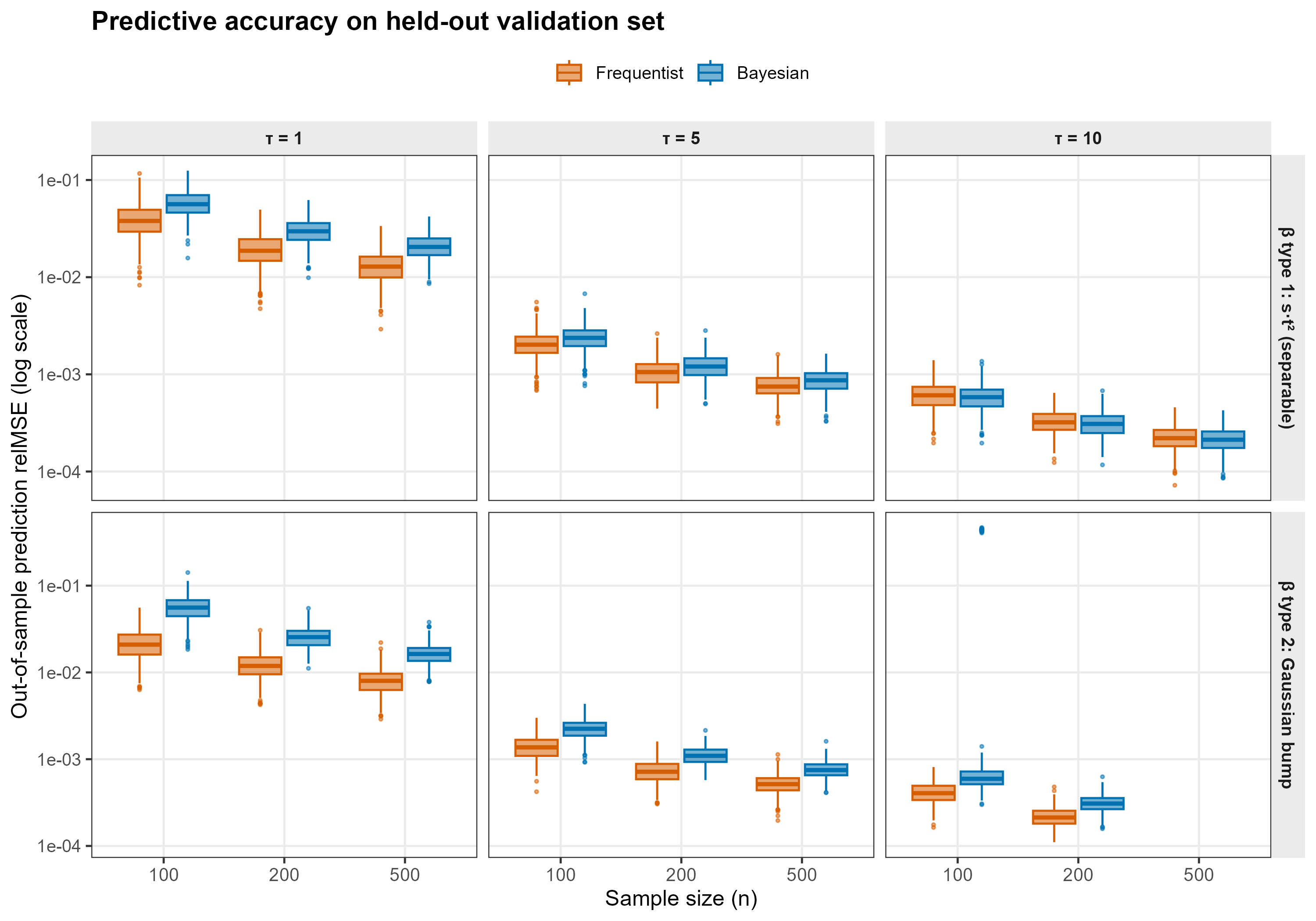
Simulation Study: Bayesian vs Frequentist FoFR

To benchmark fofr_bayes() against the standard frequentist function-on-function regression fit, we ran a simulation study comparing posterior-mean prediction against the penalised tensor-product estimator implemented in refund::pffr(). The full simulation script is shipped as Simulation/FoFR_Simulation_V3.R, with a stand-alone Stan program in Simulation/StanFoFR_Gaussian.stan.

Simulation Setup

Functional observations were generated from a function-on-function model without scalar predictors:

$$Y_i(t_m) \;=\; \frac{1}{L}\sum_{l=1}^{L} W_i(s_l)\,\beta_{\text{true}}(s_l, t_m) \;+\; \epsilon_i(t_m), \qquad \epsilon_i(t_m) \stackrel{\text{iid}}{\sim} N(0, 0.5^2),$$

on uniform grids of size $L = M = 30$ over $[0, 1]$. Functional predictors $W_i(s)$ were generated as four-component Fourier expansions with eigenvalues $(2.5, 2.5, 2.5, 2.5)$. Two true bivariate-coefficient surfaces and three signal-strength levels were considered:

Factor	Levels
Sample size $n$	$100,\; 200,\; 500$
$\beta$-surface type	type 1: separable $\beta_{\text{true}}(s,t) = \tau\,s\,t^2$; type 2: Gaussian bump $\beta_{\text{true}}(s,t) = \tau\,\exp\{-5[(s-0.5)^2 + (t-0.5)^2]\}$
Signal-strength multiplier $\tau$	$1,\; 5,\; 10$

Each cell of the $3 \times 2 \times 3 = 18$ design was replicated approximately 500 times, giving roughly 9000 fits per method.

Comparator Methods

• Frequentist baseline – refund::pffr() with a single ff(X_func, xind = sgrid, integration = "riemann", splinepars = list(bs = "ps", k = c(10, 10))) term and the response indexed by yind = tgrid. The integration = "riemann" option is critical here: the data-generating quadrature is left-Riemann with uniform weight $1/L$, and matching this in pffr() (rather than the default Simpson rule) keeps $\hat{\beta}$ on the same pointwise scale as $\beta_{\text{true}}$ during recovery comparisons.
• Bayesian model – refundBayes::fofr_bayes() (or the equivalent standalone Stan program in Simulation/StanFoFR_Gaussian.stan), with k = 10 predictor-domain cubic-regression splines, spline_df = 10 response-domain B-splines, FPCA residual structure estimated via refund::fpca.sc(), 1 chain, 1000 iterations (500 warm-up).

Performance Metric

For each replicate we draw an independent validation set of $n_{\text{valid}} = 5000$ subjects from the same data-generating process, evaluate each method’s predicted mean response $\widehat{\mu}_i^{\text{val}}(t)$, and compute the relative prediction MSE

$$\text{relMSE}^{\text{pred}} \;=\; \frac{\frac{1}{n_{\text{valid}} M}\,\sum_{i,m}\bigl\{\widehat{\mu}_i^{\text{val}}(t_m) - \mu_i^{\text{val}}(t_m)\bigr\}^2}{\frac{1}{n_{\text{valid}} M}\,\sum_{i,m}\bigl\{\mu_i^{\text{val}}(t_m)\bigr\}^2}.$$

This metric is invariant to the unidentifiable additive-in-$t$ component of $\beta(s, t)$ (see the package’s Simulation/FoFR_identifiability_note.md for details), so it provides an apples-to-apples comparison even though pffr() includes an explicit functional intercept and fofr_bayes() does not.

Results

FoFR predictive accuracy

References

• Jiang, Z., Crainiceanu, C., and Cui, E. (2025). Tutorial on Bayesian Functional Regression Using Stan. Statistics in Medicine, 44(20–22), e70265.
• Crainiceanu, C. M., Goldsmith, J., Leroux, A., and Cui, E. (2024). Functional Data Analysis with R. CRC Press.
• Goldsmith, J., Zipunnikov, V., and Schrack, J. (2015). Generalized Multilevel Function-on-Scalar Regression and Principal Component Analysis. Biometrics, 71(2), 344–353.
• Ramsay, J. O. and Silverman, B. W. (2005). Functional Data Analysis, 2nd Edition. Springer.
• Ivanescu, A. E., Staicu, A.-M., Scheipl, F., and Greven, S. (2015). Penalized Function-on-Function Regression. Computational Statistics, 30(2), 539–568.
• Scheipl, F., Staicu, A.-M., and Greven, S. (2015). Functional Additive Mixed Models. Journal of Computational and Graphical Statistics, 24(2), 477–501.
• Carpenter, B., Gelman, A., Hoffman, M. D., et al. (2017). Stan: A Probabilistic Programming Language. Journal of Statistical Software, 76(1), 1–32.